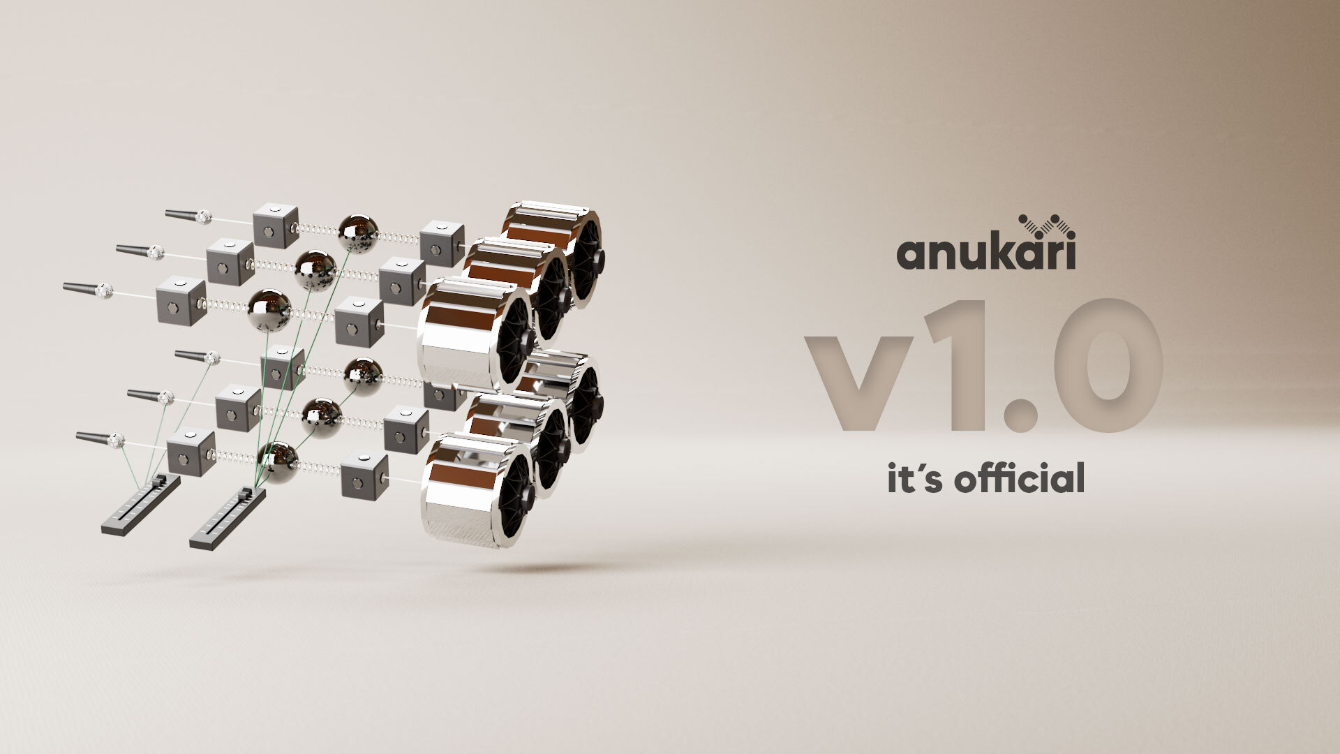
Anukari 1.0 is out. Reflections on three years of full-time work, from leaving Google and a broken shoulder to first sound and full polyphony.
Evan Mezeske
Jun 2026
Stories from my Meebo years, including the HR outage that made Trampoline Enthusiast my official job title and the great finger rocket wars.
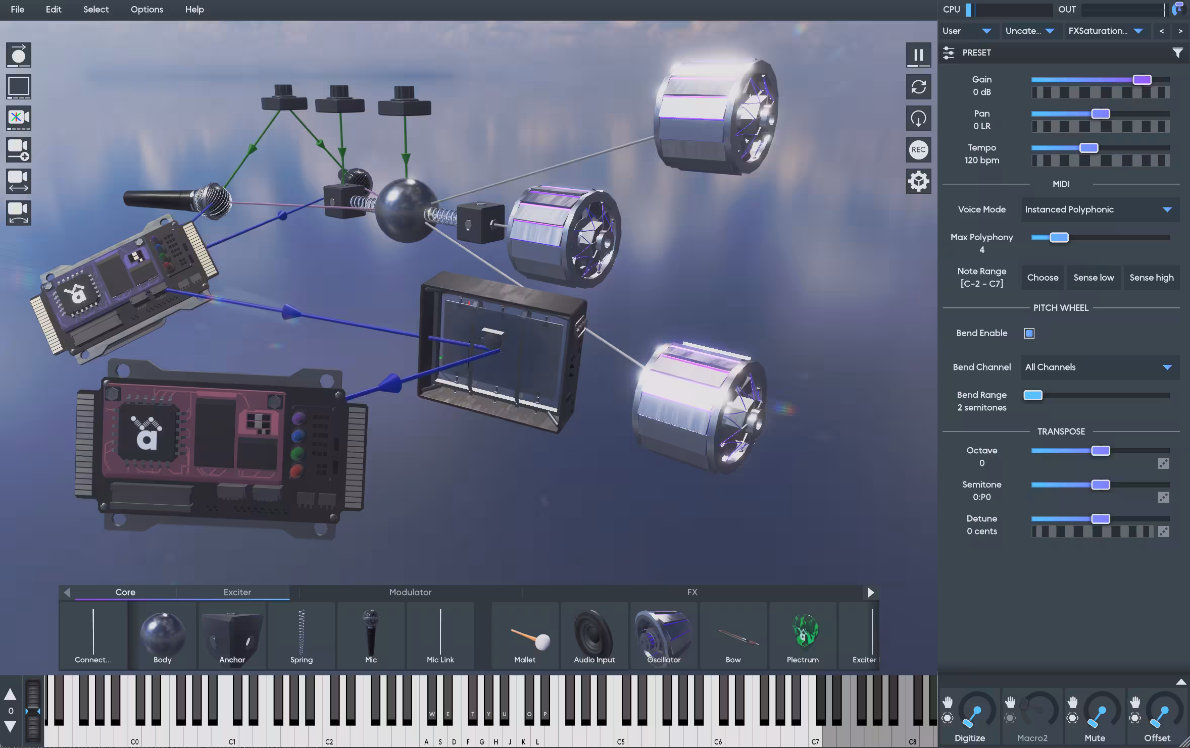
The new FX object puts 27 effects like reverb and vocoder in the 3D scene, instanced per voice so the FX chain can feed back into the physics.
Claude handles the incidental complexity now, so I cleared a pile of long-stalled UX tasks like parameter smoothing, plus thoughts on coding with AI.
Why I replaced Google Filament with 40K lines of custom PBR engine code, written with Claude in weeks, that survives VK_DEVICE_LOST without crashing.
Release 0.9.30 adds post-processing shaders and 1-click screen recording. The recorder alone is 6,500 lines of platform-specific C++, built with Claude.
Mar 2026
How 0.9.26 cuts Anukari's RAM use. A lock-free background allocator with epoch-based freeing replaces 154 MB of preallocated delay line buffers.
Resend's global suppression list was silently eating my customers' license key emails, so I migrated anukari.com to Postmark for deliverability.
Feb 2026
MTS-ESP microtuning support landed in an afternoon, alongside NAMM followups, an AU validation hang fix, and a Filament reflections crash on AMD.
A custom votive candle of DSP legend Julius O. Smith III led to meeting Nicholas Porcaro and Pat Scandalis at the Anukari NAMM booth.
I replaced the crackling JUCE limiter with a hard limit at +6 dBFS and re-leveled all 200+ factory presets to -15 LUFS for far more dynamic range.
Dec 2025
After Railway's software audit policy and Northflank's broken 503-throwing proxy, anukari.com now runs on Cloud Run behind a global load balancer.
Railway blocked my emergency deploy over dependency CVEs already live in prod, and why piling on safety checks eventually causes the outage.
Looking back at the GPU years, where my 50,000-object goal led me astray, and why one SIMD backend beats maintaining CUDA, Metal, and OpenCL.
Nov 2025
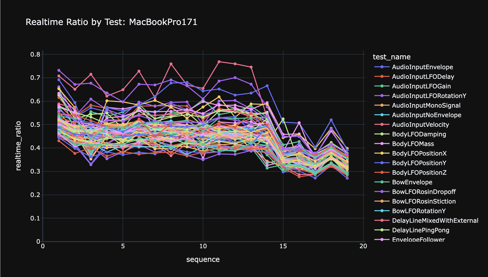
Part 2 of the CPU rewrite, from spot-vectorizing float3 math with SSE and NEON intrinsics to restructuring loops for compiler auto-vectorization.
Anukari now runs on the CPU with hand-coded SIMD instead of the GPU. Part 1 explains the GPU origin story and the naive port that was only 5x slower.
Eight mappable macro knobs land in the UI with drag-and-drop modulation binding, plus 312ears built a Python preset API from my protobuf definitions.
Aug 2025
The Radeon gfx90c driver aborts in clBuildProgram because it can't index kernel argument arrays dynamically. Moving them to constant memory fixed it.
Jul 2025
Multichannel 50x50 audio I/O with near-zero overhead, ASIO support on Windows, and a workaround for a Radeon clBuildProgram crash on gfx90c.
With Apple's help I cut Metal kernel launch overhead under 50us using MTLSharedEvent and double-buffered encoding, then had to unbreak CUDA.
May 2025
Applying Apple's NDA guidance to the GPU spin loop, serializing its kernels with MTLEvent, and deduplicating it across processes via shared memory.
My Appeal to Apple post worked. I got a call with a Metal engineer, performance hints I can use now, and an open line to the right people at Apple.
macOS GPU clock heuristics don't recognize real-time audio work, and my spin loop workaround fails on Pro and Max chips. I need the Metal team's help.
Demo mode now ducks the output gain instead of blasting white noise, plus a first-launch flow with a skin picker and a near-instant preset chooser.
Apr 2025
With 85 factory presets and a preset maker contracted, I'm prepping the first public release. Payments will go through Shopify, app store gripes included.
Mar 2025
Porting Anukari to AAX went smoothly aside from the iLok and PACE signing dance, and Pro Tools flushed out bugs that also affected VST3 and AU.
Feb 2025
An undocumented Metal error 14 with multiple plugin instances traced to kernels clearing 300 MB delay buffers that a low-watermark check made unnecessary.
GarageBand silently stops calling ProcessBlock, so Anukari now detects the auto-bypass and hands the physics simulation to a background thread.
I ditched CPack's crippled installer generators for Inno Setup and pkgbuild directly, and shipped a new AnukariEffect plugin for use in effect chains.
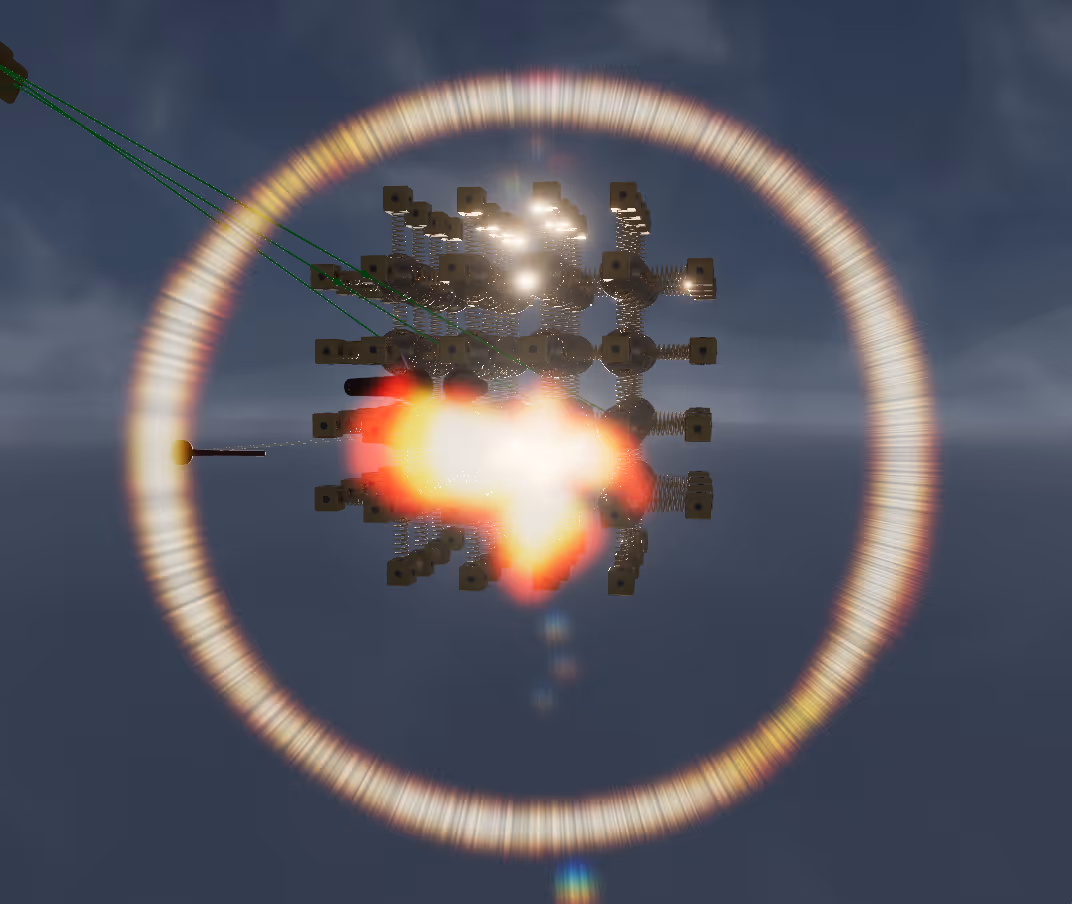
Physics explosions from oversized time steps now get auto-mitigated, with the GPU tracking peak velocity and silently resetting any voice that blows up.
Jan 2025
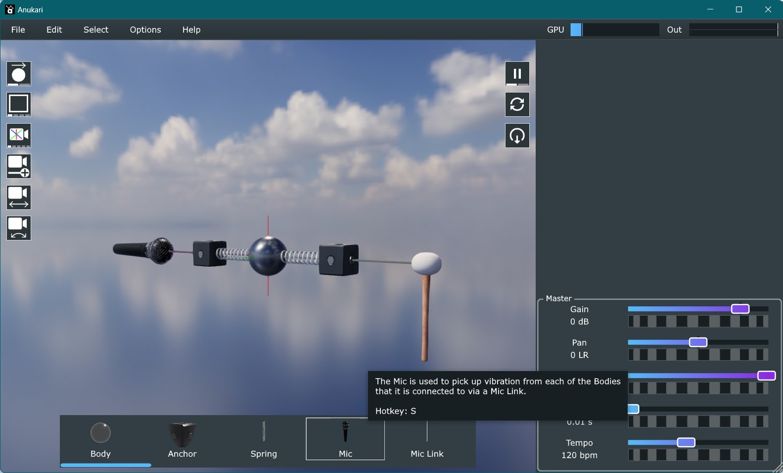
A draggable entity palette with live-rendered thumbnails, color-coded connection highlighting, and camera icons that make the 3D controls discoverable.
Dec 2024
I built a chaos monkey that hammers Anukari's GUI with random pyautogui input. It found crashes I'd never have tested and ran 10 hours clean.
Custom 3D models broke my hard-coded hitboxes, so mouse picking now runs on Bullet Physics raycasts against convex hulls approximating the model geometry.
Nov 2024
A minimax optimizer now packs Anukari's 11 entity types into 32 GPU warps to minimize branch divergence. Huge presets run up to 2x faster.
The CUDA port is done with all goldens passing. Native 1024-thread blocks beat OpenCL's 256-thread cap, so big presets no longer double their latency.
MacOS won't up-clock the GPU for latency-sensitive audio, so Anukari now burns one warp on useless spin work. Latency dropped about 40 percent.
Metal profiling shows the simulation is ALU-bound, so I'm chasing half floats and signed indexes, plus a visual style doc for hiring 3D artists.
After emailing DAW makers for NFR licenses I got Anukari stable in 13 hosts, fixing a Bitwig native window crash and a SymInitialize crash in Sonar.
Oct 2024
Random glitches on the Filament Metal backend came down to render passes without a color clear. Enabling clearing fixed it and I filed an upstream bug.
Ableton's Auto-Scale Plug-In Window option sent me down the Windows DPI awareness rabbit hole and into a Vulkan swap chain scaling driver bug.
Async background asset loading plus a detachable cached renderer make reopening Anukari's VST GUI instant, even with 256 MB 2K skyboxes.
Skyboxes and lighting are now zip-file presets anyone can build from an .hdr file, and the instrument's 3D models load from swappable .glb presets too.
Filament now builds as a git submodule inside Anukari's CMake, and the renderer preferences menu has low, medium, high, and max speed presets.
Tracked down a JUCE bug duplicating mouse events between stacked NSViews on macOS, plus a Filament black screen on Intel Iris Xe OpenGL.
Window resize crashes traced to Filament's Vulkan backend never destroying swap chains, plus a JUCE macOS bug where mouse hover flickers between windows.
I wired render-thread errors into the GUI thread and redid the camera controls, with rotate on right-click drag and pan on shift so touchpads work.
Filament's JIT shader compilation was the whole startup delay, so I switched to ubershaders. The floating GUI now uses native OS child windows.
Bodies scale with mass, springs thicken with stiffness and redden with tension, and links light up with signal. Also fought Filament's messy cleanup APIs.
The Filament renderer now matches the old OpenGL one, selection highlights and all. I deleted the hand-rolled renderer and fixed the Windows file browser.
Ableton destroys the plugin window before the editor, crashing Filament's Vulkan swap chain. Hooking WM_DESTROY to shut the renderer down first fixed it.
Sep 2024
A hacked-together skybox and irradiance map give the .glb objects environmental lighting, and masses and springs finally look right again.
Filament now draws my Blender models as instanced .glb assets and gives me shadows and ambient occlusion for free. Asset caching is next.
The new renderer runs on macOS via Metal and an NSView overlay, with OpenGL fully removed. The macOS audio performance mystery remains unsolved.
After a dead end with WS_EX_LAYERED transparency, I'm drawing the 3D graphics in an HWND on top of the JUCE GUI, and native popup menus still appear.
Getting Filament rendering into a JUCE window is harder than expected since JUCE hides its swap chain, and overlay native windows break menus.
On macOS the 3D graphics interfere with GPU audio even when nothing is drawn, so I'm starting the Filament port to rule out Apple's OpenGL.
The OpenCL kernel now compiles and runs under Metal via macros and passes the golden tests, though the rough port still leaks memory everywhere.
Split the simulator into a shared base with OpenCL and Metal children. Macros may let the same kernel source compile for OpenCL, Metal, and CUDA.
The GPU copy optimization landed well, and NVIDIA on Windows runs big presets fine, but MacOS OpenCL stays mysteriously memory-bound. Metal port is next.
Aug 2024
Moving final microphone mixing onto the GPU should slash CPU-GPU copy bandwidth, my plan for the Mac performance problems pre-alpha testers uncovered.
Windows and MacOS installers finally work on other people's machines, after switching back to Apple Clang and a vcpkg triplet targeting MacOS 11.
Windows pre-alpha is solid, so now I'm chasing MacOS bugs like file chooser corruption, plus a pkg installer since a dmg can't place VST3 and AU files.
One button now builds a signed Windows installer via CPack, EV certificate, EULA screen and clean uninstall included. MacOS packaging is next.
License activation C++ is in, and instead of mocking HTTP I wrote integration tests that hit the real license server with a test-only reset API.
Pre-alpha builds now download via short-lived Cloudflare R2 URLs so leaks go stale fast, plus license key verification in C++ and a round of vcpkg pain.
The devlog and newsletter now live on anukari.com, imported from Discord and Substack, which I'm shutting down. Pre-alpha invite tooling is next.
I built the site's blog engine, imported the old Discord devlog entries, added tagging and RSS, and wired a bot to pipe new posts back into Discord.
A missing await on an async function led me to typescript-eslint's promise rules, which surfaced a dozen similar bugs in the new website's code.
Moving MongoDB index creation into version-controlled TypeScript, then hitting a next.js bug where failed middleware makes server actions return undefined.
The licensing API is done. The plugin sends a machine fingerprint plus license key and the server signs it back, a simple lock on the front door.
Auth, server-validated React form actions, and CSRF protection are working, so I'm pushing the website toward pre-alpha product key management.
Jul 2024
Six hours fighting next-auth.js to get email and password login working for product registration, since the docs push everyone toward OAuth.
After boost's interval library threw baffling singleton exceptions in my GUI fuzz tests, I replaced it with a 25-line Interval class that just works.
Making Exciter velocity sensitivity adjustable took an hour, then making the 3D animations track fully modulated loudness ate the rest of the day.
Fixed the clanking when raising the voice instance slider (init state wasn't stored per-instance) and added MIDI note off velocity as a modulation source.
Voice stealing now prefers released notes, which made MPE playable when holding a root note under a melody. Lots of polyphony GUI details cleaned up too.
Porting the whole website from Python to next.js took about three hours, and JSX plus React components beat every Python templating option I have tried.
Google Cloud Run made mapping a custom domain such a slog that I moved the site to railway.app, which had it serving in five minutes. NiceGUI is out too.
Plugged in the ROLI Seaboard and MPE just worked, two notes bending in opposite directions. Also switched the new website from App Engine to Cloud Run.
MPE is implemented, including storing per-channel pitch, pressure, and CC74 between notes. Untested since my Seaboard came without the right USB cable.
Spent the day on a new website in Python, FastAPI, and NiceGUI on App Engine, and landed on a three word tagline for Anukari, 3D Physics Synthesizer.
MPE zones, channel counts, and pitch bend ranges are in the data model now, and the global pitch wheel bends any preset via time dilation.
With polyphony working well, I'm starting on MPE support ahead of my ROLI Seaboard's arrival, including the annoying MCM zone auto-configuration messages.
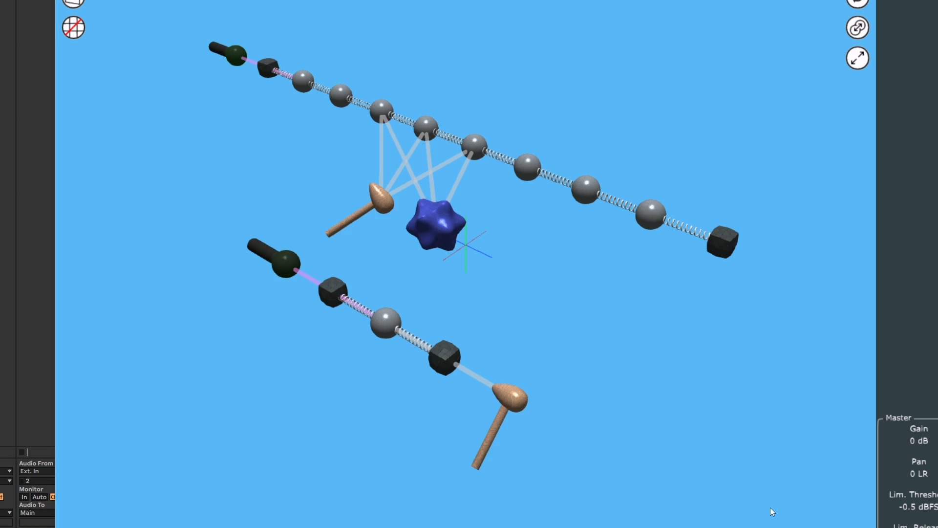
Voice instancing works and it's better than I hoped. Time dilation retunes a full physics sim per note, and parallel GPU voices add zero slowdown.
Reworking the data model so MIDI and modulation state can be stored per voice instance, groundwork that MPE support will build on directly.
With code signing done and the macOS port shelved for now, I'm back on voice-instanced physics, running parallel instrument copies in OpenCL.
Wrestling with code signing bureaucracy, from Apple Developer verification and D-U-N-S numbers to picking a Sectigo certificate for Windows binaries.
Jun 2024
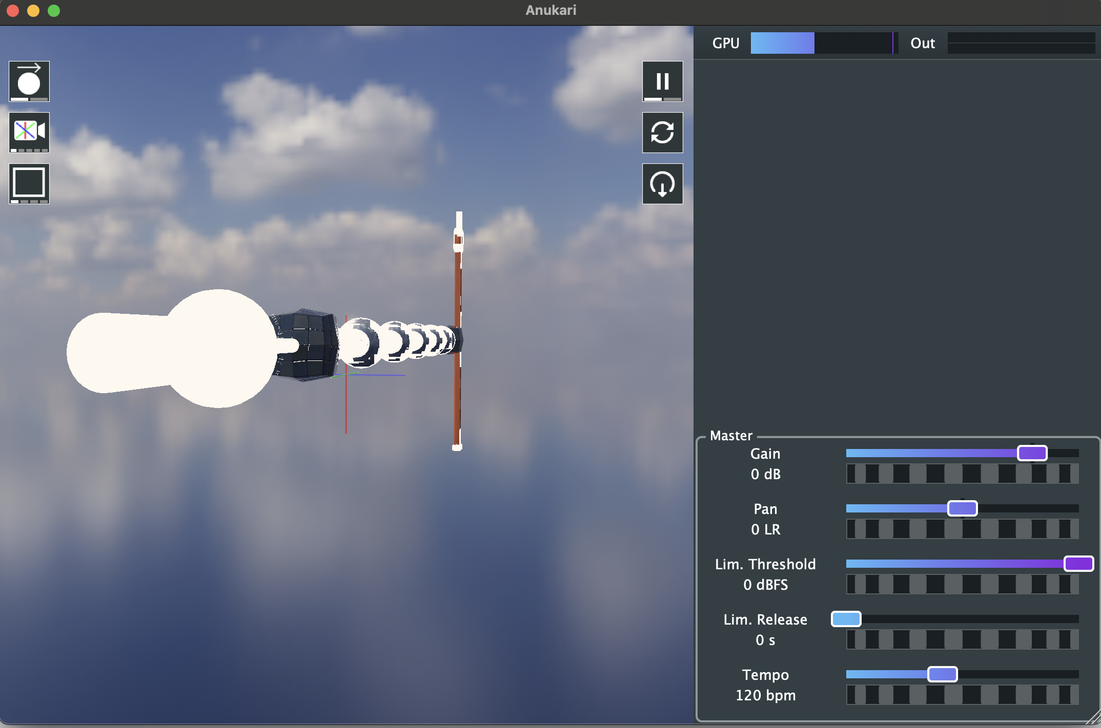
Anukari's standalone build is now fully usable on MacOS, with the GUI, MIDI input, audio output, and hotkeys working after a morning of small bug fixes.
Golden tests now compare audio via chunked FFTs and L2 distance, which surfaced an OpenCL bug on Mac where objects can legally live at address NULL.
After cleaning up the macOS port hacks and re-verifying Windows, Anukari now runs fully on my M1 MacBook, though the golden tests need fuzzy matching.
JUCE resists testable apps, so on macOS I moved all the unit tests inside a full JUCEApplication, trading test isolation for tests that pass.
Back from paragliding and porting unit tests to MacOS, which forced a cleaner cross-platform approach to GUI testing than my hacky Windows-only setup.
Anukari finally builds and links on my M1 Macbook after homebrew Clang pain, though the OpenCL code crashes whenever a microphone or modulator appears.
Two voice instances now run in parallel GPU work groups and pass the golden tests. Links stay shared in memory, so only mutable entities duplicate.
May 2024
Most of the CPU-side refactor for the new voice instancing memory layout is done, with golden tests catching every break in the CPU-to-GPU data reshuffle.
Breaking ground on instanced voice mode, which turns any instrument polyphonic by using time dilation for tuning. Prototype first, design later.
My copy-paste fuzz test caught a subtle bug where links that connect to other links pasted in the wrong order, breaking the two-pass materialization.
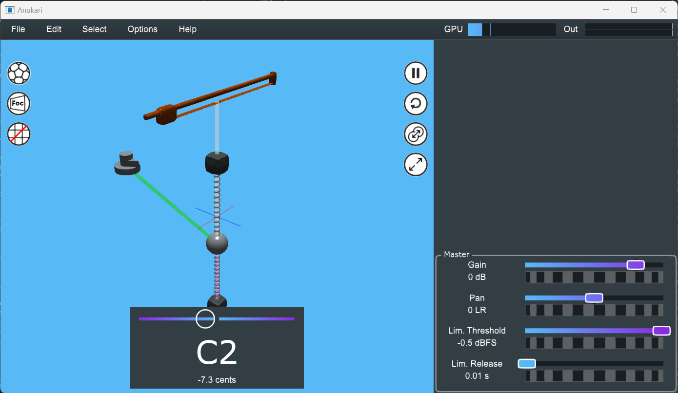
Anukari has a built-in tuner now. After wading through GPL-licensed and broken pitch estimation libraries, I settled on cycfi's q, fast and stable.
Copy and paste handles link and MIDI route edge cases now, backed by a fuzz test that pastes random entity subsets 10,000 times and checks invariants.
Paste, duplicate and import now use AABB search to land entities in clear space, and simulator reset became trivial via full serialize and reload.
The Audio Units logo and the Audio Units symbol are trademarks of Apple Computer, Inc.
VST is a trademark of Steinberg Media Technologies GmbH, registered in Europe and other countries.


.jpg)